The Bias in Allocation Profiling
I’m very exciting about reviving my blog and launching my first real post. There are a bunch of quotes on the subject of measurements. The two I like to focus on are “You can’t improve what you don’t measure” (Peter Drucker) and “we are only as good as our measurements”. The problem with measurements is that they are all flawed in some fundamental way. Our measurements may be lacking in some combination of precision, or accuracy. We may be measuring at the wrong resolution. Maybe we can’t measure everything so instead we sample. If we do sample, then we need to pick our bias because ever sampling technique comes with some form of bias. This bias will skew our measurements and consequently, our interpretation of the system we are measuring. This is the basis for the theme here, how the bias in how allocation profilers measure affect our ideas of how. we can improve the memory efficiency of our applications and how having multiple perspectives, or measurements might provide us with a truer picture.
The impact of allocation pressure on application performance cannot be understated. In my experience, and the experiences of others that I’ve spoken to about this is that, reducing allocation pressure can result in whole integer improvements in performance. Often this can happen with seemingly small changes to the application. Why can we get these huge performance wins by reducing allocations? The quick answer is because the performance of an application with a high allocation rate is almost always dominated by cache misses. For the longer answer this question, we will take a shallow dive into the relevant bits of the tech stack and then take a look at the biases in allocation profilers.
Some Hardware Bits
When the CPU needs to load a data value into a register, it first searches for it in each of the CPU caches. Not finding the data in the CPU cache is known as a cache miss. A cache miss triggers the CPU to issue a fetch to main memory. The high-level description is that the fetch request is transmitted across a bus to main memory where the controller works out which memory needs to be read, reads it and then returns it back to the CPU on the bus. The data is then dragged through the CPU caches, through the load buffer and finally into the target register. While all of this is happening, the thread that referenced the data will be stalled. Typical stalls last a couple hundreds of clocks. In comparison, finding the data in the L1 cache will take 4 clocks and maybe less if the CPU has been able to pre-fetch. How does this tie into allocations?
Allocations in Java
One of the jobs of the Java Virtual Machine (JVM) is tasked with is to manage memory. To manage this, the JVM includes several different data structures and algorithms that work together to provide this critical functionality. This includes Java heap, the garbage collector, and the algorithms that orchestrate allocations. I won’t be describing any of these components in detail but instead will be focusing on the bits that are important to the topic at hand.
Allocations in Java heap use a technique known as bump and run on a head of heap pointer. As can be seen in the diagram below, the head of heap pointer points to the top of all of the data that has been allocated.
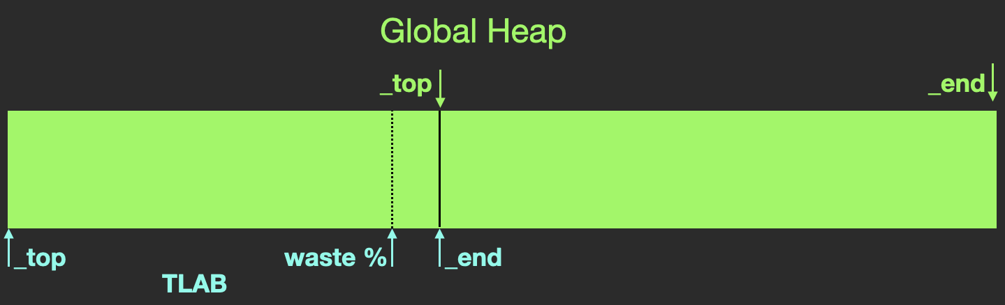
TLAB allocated from Global Java Heap
To “bump and run” the pointer must first be loaded into a register. This value is then incremented by the number of bytes needed to satisfy the needs of the allocation after which the thread can continue to run. Given that just about all Java applications have multiple threads allocating at the same time, the head of heap pointer will need to be wrapped in a lock to ensure mutual exclusive access. This naive implementation comes with a number of high latency activities. First, the cost of the barriers needed to insure that the view of the pointer value is consistent across all threads is the equivalent of a cache miss. Next, the lock necessarily serializes all allocation activity. In the, very likely, case where the head of heap pointer is highly contented, allocating threads would be backed up into a queue waiting for their turn to be able to allocate. Enter Thread Local Allocation Block (TLAB). TLABs act to reduce the pressure on the head of heap pointer. Let’s spend a bit of time exploring how this works.
When a thread allocates, the allocators will check to see if the thread needs a new TLAB. If so, a new TLAB will be allocated in Java heap by bumping up the global head of heap pointer. TLAB size starts at 1MiB and the head of TLAB will be at 0 relative to the base address of the TLAB. TLAB size can and does vary as it is adaptive to allocation pressure but we can be ignore this feature for the purposes of this discussion. The more salient point is that the TLAB forms a new allocation buffer that is only visible to the thread that allocated it. To continue with the allocation story, now that the thread has a TLAB, the thread can bump a head of TLAB pointer to complete the allocation. Of course, this pointer bump is un-contented which significantly improves the allocation performance. However, there is no free lunch as using TLABs does result in more memory being wasted. To better understand this, let’s look at a couple of allocation use cases.
TLABs have a configurable waste percentage setting. The purpose of this waste percentage is to set a boundary. At the beginning of an allocation, the allocator checks to see if the current head of TLAB is past the boundary and if so, the thread is obliged to allocate a new TLAB. The allocation will then complete in that new TLAB. This implies that the memory between the head and the top of the TLAB will never be used. The next case to consider is when the head of TLAB is below the waste threshold but the size of the allocation would overflow the TLAB. In this is quite different then when the head of TLABan allocation + head of TLAB would result in a buffer overrun. In that case, the allocation will happen outside of the TLAB in the global heap space. This use case implies that allocations bigger than the TLAB will happen in the global heap space. A more subtle effect is that the size of globally allocated objects will decrease as the TLAB fills up. The relevance of this last point will become more apparent very shortly.
Returning to the subject of cache misses, what is evident from the description above is that an allocation is Java heap (or a TLAB) is realized though the manipulation of a data structure where the elements of that data structure have never been or not recently been referenced by the application. This suggests that the needed part of the data structure will not be in any of the CPUs caches. With high allocation rates, it is very likely that even if the needed part of the data structure was accessed recently, the motion of data churning through the cache would have resulted in it being flushed. Fortunately the JVM offers some help.
One of the optimizations that the Just-in-Time (JIT) C2 optimizing compiler is able to provide is known as scalar replacement. Very briefly, scalar replacement literally replaces an allocation call site with the assembly code that has the field value inlined instead of being stored in Java heap. As you can imagine, this optimization comes with a lot of restrictions one of the most important is that the allocation passes the Escape Analysis (EA)test. EA determines the visibility of object produced by the call site to be scalar replaced (also known as a call site reduction). There are 3 outcomes for this test, fully escaped meaning the data is visible to multiple threads, partial escape meaning the data maybe visible to other threads, or no escape meaning that the data is only visible to the thread that created it. For example, any variable labeled public is at least partially escaped if not fully escaped whereas any variable that remains completely local to a specific code block would most likely be no-escape. There are other constraints but it’s safe to say that many allocations can be eliminated with this optimization. The win is that the thread is able to avoid the cache miss that comes with the on heap allocation.
One more sidebar, profilers commonly report on allocation rate as bytes/sec. As can be seen from the description provided so far, the size of the allocation is a minor factor if it even is a factor at all in the cost of an allocation when compared to the cost of a cache miss. Thus the bytes/sec reporting isn’t all that useful when we’re looking for the number of allocations/sec.
With all this in mind, let’s take a swing at allocation profiling.
Allocation Profiling
There are a several ways to implement an object profiler. Way back in the days of Java 1.1.7, I whipped up an allocation profiler that reported on the allocation to a table. It was simple and effective but it inflicted a horrendous overhead penalty on the application. Today, profilers tend to wrap the allocation in a phantom reference. The profile harvests and reports on information harvested from the phantom reference. While these profilers offer far less overhead than my hacked up tool did, it is still not insignificant. The other big effect is on EA. Wrapping the allocation in a PhantomReference to be processed by the profiler means that the data is accessible by more than 1 thread and thus EA will label it fully escaped. Thus a consequence of using this technique is that ALL allocations will fail EA.
The next course of action is to inspect the profiler output for the hottest allocation site, optimize the code to either remove or reduce it, then rerun the performance tests and report on the improvement. Sound good but what happens fairly frequently is that the test produce no noticeable reduction in latencies. While there could be many reasons for this a common one is that the hottest allocate site was already being optimized by the JIT resulting in the “fixes” to the code being redundant. This is where tools like JITWatch can help. This tool will report on allocation sites that have been scalar replaced. Comparing this list to the profile can help you pick hot allocation sites that are not being optimized away.
The other technique is to sample out-of-TLAB allocations and those allocations that trigger the creation of a new TLAB. In JFR the code perform this is baked into the JVM so the overhead is fairly minimal. To be honest, I’m not sure how the async-profiler collects this data though I suspect it is by capturing the JFR event. This is something I plan on looking into in the near future.
While on paper TLAB sampling may look ok, in practice it biases the profile to large allocations. Indeed if you profile an application that allocates an equal number of various sized objects and plot that data this bias will become immediately obvious. The smaller objects will be under reported whereas the larger objects will be over-reported. Again, being mindful of purpose, we’re looking for the rate at which objects are being allocated, not the rate at which memory is being allocated. In this case I can only offer 1 solution and that is to turn off the use of TLABs while profiling. If you’re thinking that according to the description above thats going to degrade performance the answer is yes, it’s going to hurt. However, missing that it’s a small allocation that is escaping that is the source of your allocation pressure isn’t all that helpful either.
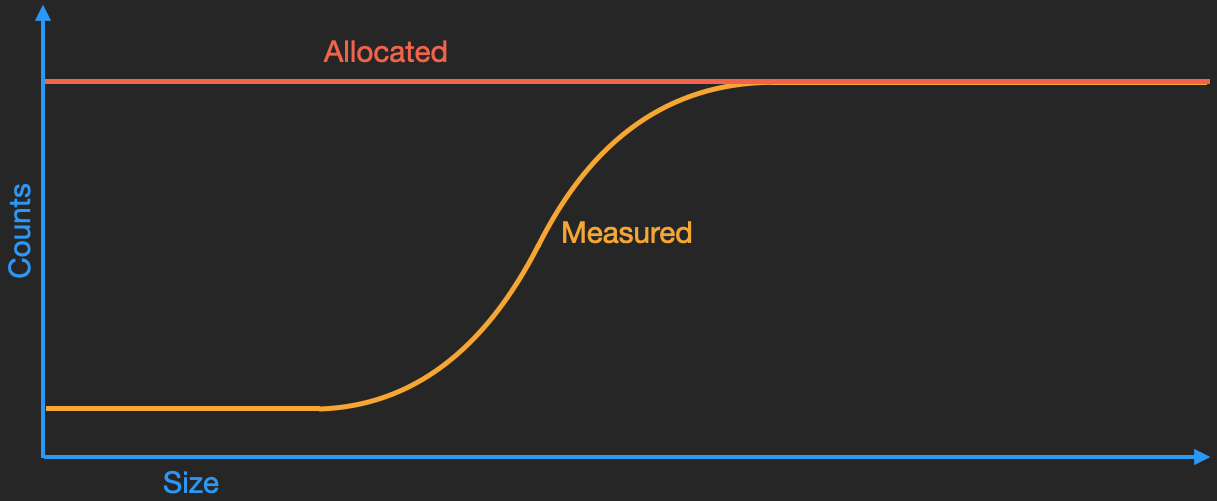
Allocation True Counts vs Sampled Counts
What about Heap Dumps
I’ve heard several people advocate the use of heap dumps in finding hot allocation sites. My personal view point is that finding a hot allocation site with a heap dump is even more problematic than the challenges thrown at by the traditional allocation profilers. About the only recipe that I’ve heard, but have not tried, it to use the Epsilon collector (or otherwise turn off GC) and trigger a heap dump after running some load on the application. The next step is to use a heap analysis tool to inventory the entire contents of the heap dump. This would necessarily include both live and dereferenced objects.
Conclusion
As is evident, each of the profiling techniques in use today come with upsides and downsides. A quick summary of this is that the upsides for JFR are very low overhead and convenience. The downside is the bias towards large allocations. The async profiler isn’t as convenient to use but it also offers low overheads with the bias towards large allocations. On the other side of the spectrum, tools like VisualVM record every allocation but unfortunately not easy to deploy in prod (-like environments), interfere with EA and come with a high overhead. On the question of which profiler should one use? I tend to use all of them (including commercial options that I’ve not listed here). But, which on you should use really depends on your situation. Hopefully the information offered here can help you in that decision making process.